Go to CCP Homepage Go to Materials Page Go to Linear Algebra Materials Go to Table of Contents
Go Back One Page Go Forward One Page

Curve Fitting

Part 3:  Linearization

It is common practice to try to fit non-linear models to data by first applying some transformation to the model that "linearizes" it. For example, suppose we want to fit the non-linear exponential model

y = a ebt

to the U.S. population data from Part 1.  The standard trick is to linearize the model by taking logs:

ln(y) = ln(a) + b t.

Now we have a model in which the parameters A = ln(a) and b appear linearly. We can fit a least squares line to the data

(T1, ln(Y1) ) ),  (T2, ln(Y2) ), ... ,  (T10, ln(Y10) ).

That is, we fit a least squares line to the semi-log plot of ln(y) versus t shown below.
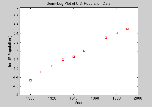
Semi-log plot of U.S. Population data


  1. For the U.S. population data, the vectors

    y* = ( ln(Y1), ln(Y2), ..., ln(Y10) )T,

    t =  ( T1, T2, ..., T10 )T ,

    and
    1 = (1, 1, ..., 1)T

    are defined in your helper application worksheet.  Solve the normal equations for the parameters A = ln(a) and b of best fit and then find the best fitting exponential model y = a ebt.

  2. Plot the exponential function that you just found together with a scatter plot of the original U.S. Population data (not the logarithms).  How good is the fit?

  3. Compute the residuals y - p and the sum of squares S of the residuals. Make a residual plot.  What do you learn from the plot about the goodness of fit?


  4. Compare the fit of the exponential model to the quadratic model of Part 1.  You should have already computed S for the the quadratic model. You should also make a residual plot for the quadratic model for comparison purposes.


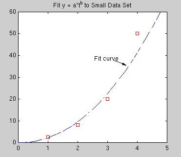
Small Data Set
t
y
 1.0 2.5
 2.0 8.0
 3.0  19.9
 4.0  50.0
Scatter plot of small data set

Above is a small data set.  Let's try to fit this data with a power function of the form

y = a tb

by first linearizing the model by taking logs:

ln(y) = ln(a) + b ln(t).


  1. For the small data set above, the vectors

    y* = ( ln(Y1), ln(Y2), ln(Y3), ln(Y4) )T,

    t* = ( ln(T1), ln(T2), ln(T3), ln( T4) )T ,

    and
    1 = (1, 1, 1, 1)T

    are defined in your helper application worksheet. Fit a line to the log-log (ln(Ti), ln(Yi)) data and use the results to find the model parameters for the corresponding power function y = a tb

  2. Plot the power function that you just found together with a scatter plot of the original small data set (not the log-log plot).  How good is the fit?

  3. Compute the residuals y - p and the sum of squares S of the residuals. Make a residual plot.  What do you learn from the plot about the goodness of fit?


Go to CCP Homepage Go to Materials Page Go to Linear Algebra Materials Go to Table of Contents
Go Back One Page Go Forward One Page


modules at math.duke.edu