Part 2:  Linear Least Squares

that is, if the model function is linear in the parameters c₁, c₂, ... , c_k of the model.  In our quadratic model of Part 1, the component functions used in defining f(t) were g₁(t) = 1, g₂(t) = t, and  g₃(t) = t².

Let's see why the method of Part I works for the more general linear model.  Suppose the data points are (T_i, Y_i), i = 1, ... , n. Define the following vectors in Rⁿ:

Then W = Span(g₁, g₂, ... , g_k) is the k-dimensional subspace of Rⁿ of vectors of the form

The least squares problem is to find values of the parameters c₁, c₂, ... , c_k that produce the vector in W closest to y.  This vector is the projection p of y onto the subspace W.

As we saw in Part 1, the values of the parameters that minimize the distance from y to W are the components of the vector
v = (c₁, c₂, ... , c_k)^T  that solves the normal equations

where X is the matrix whose columns are g₁, g₂, ... , g_k.

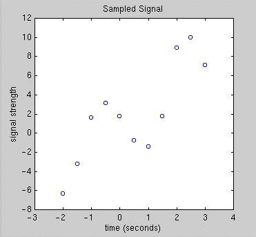
Let's look at another example.  The data below are measurements of the signal output by a small electronic device.  The signal is sampled every half second over the given time interval.  We want to find a sinusoidal model function that provides a good fit to the observed data.
 

Sampled Signal Time (sec) Signal Strength     (millivolts) -2.0 -6.32 -1.5 -3.23 -1.0  1.62 -0.5  3.13  0.0  1.74  0.5 -0.75  1.0 -1.41  1.5  1.78  2.0  8.88  2.5 9.98  3.0  7.10

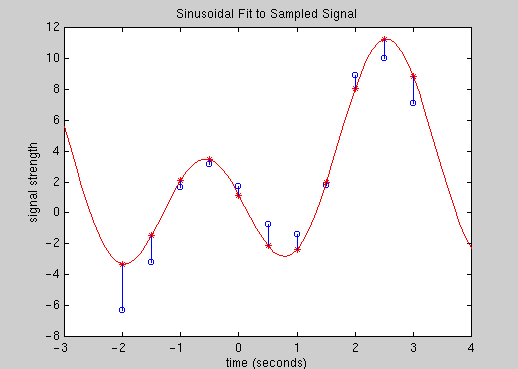
Because of theoretical considerations based on physical properties of such electronic devices, we believe that a likely model function for the given output is a trigonometric polynomial of the form

The figure below shows such a candidate function.  We want to choose the parameters a₀, a₁, b₁, a₂, and b₂, to minimize the sum of squares of the residuals, which are shown in the figure.  That is, we want the best least squares fit.

1. Using the given data, the vectors
   
   y = (Y₁, Y₂, ..., Y₁₁)^T
   s₁ =  (sin(T₁), sin(T₂), ..., sin(T₁₁) )^T ,
     c₁= (cos(T₁), cos(T₂), ..., cos(T₁₁) )^T ,
   s₂ = (sin(2T₁), sin(2T₂), ..., sin(2T₁₁) )^T ,
      c₂= (cos(2T₁), cos(2T₂), ..., cos(2T₁₁) )^T , and 1 = (1, 1, ..., 1)^T

   are defined in your helper application worksheet.  Solve the normal equations to find the trigonometric polynomial of best least squares fit.
    

2. Plot the least squares trig polynomial that you just found together with a scatter plot of the signal strength data.  How good is the fit?

 
3. Compute the residuals y - p and the sum of squares S of the residuals. Make a plot of the residuals versus time t.  Such a plot is called a residual plot.  What do you learn from the plot about the goodness of fit?  (Note that non-random patterns of the residuals often indicate that the model function is not an appropriate choice.)