Growth Models, Part 2

Population Growth Models

Part 2: The Natural Growth Model

The Exponential Growth Model and its Symbolic Solution

Thomas Malthus, an 18^th century English scholar, observed in an essay written in 1798 that the growth of the human population is fundamentally different from the growth of the food supply to feed that population. He wrote that the human population was growing geometrically [i.e. exponentially] while the food supply was growing arithmetically [i.e. linearly]. He concluded that left unchecked, it would only be a matter of time before the world's population would be too large to feed itself.

The first growth model we examine in this module is the one Thomas Malthus referred to in his famous essay. (In part 3 of this module we will consider a more sophisticated model for the special case of world population). Malthus' model is commonly called the natural growth model or exponential growth model. For this model we assume that the population grows at a rate that is proportional to itself. If P represents such population then the assumption of natural growth can be written symbolically as

dP/dt = k P,

where k is a positive constant.

This model has many applications besides population growth. For example, the balance in a savings account with interest compounded continuously (and no withdrawals) exhibits natural growth. In this case, the constant k is called the annual rate of interest. Also, large animal populations whose size is not constrained by environmental factors grow exponentially. In this setting, k is called the productivity rate of the population.

A quantity Q grows exponentially if the rate of growth of Q is proportional to Q itself. Another characterization of exponential growth is that the percentage or relative growth of Q, i.e. ratio of the growth rate of Q to Q, remains constant. Why are these two characterizations of exponential growth equivalent?
Give a symbolic description of the solutions of the differential equation dQ/dt = k Q. See Part 5 of the Introduction to Differential Equations for help.
Give a symbolic description of the solution to the initial value problem

dQ/dt = k Q and Q(0) = Q₀.
Legend has it that the land now occupied by the borough of Manhattan was purchased for $24.00 in 1626. Determine what the present value of the money would be if it had been placed in a savings account earning 6% annual interest compounded continuously.
Consider the initial value problem

dQ/dt = 0.2 Q and Q(0) = Q₀.
On your worksheet, plot the slope field for the differential equation, and superimpose the solution to the initial value problem for three different values of Q₀.

Testing for Exponential Growth

The following table lists the population of the city of Houston, Texas ( county metropolitan statistical area) from the year 1850 to 1980.

Population of Houston Area

Census Date	Population
1850	18,632
1860	35,442
1870	49.986
1880	71,316
1890	86,224
1900	134,600
1910	185,654
1920	272,475
1930	455,570
1940	646,869
1950	947,500
1960	1,430,394
1970	1,999,316
1980	2,905,334

The population data of Houston have been entered into your worksheet. Plot the data. Does the growth look exponential?

In describing the character of human population growth Malthus wrote,

"A thousand millions are just as easily doubled every 25 years by the power of population as a thousand. But the food to support the increase from the greater number will by no means be obtained with the same facility".

In other words, Malthus is claiming that, for a population undergoing exponential growth, the time it takes to double is independent of the size of the population.

Suppose the current population is P₀ = P(t₀). Let P be the solution to the initial value problem dP/dt = kP, P(t₀) = P₀, that is, P(t) = C e^kt for some constant C. Find the doubling time T, i.e., the time T such that P(t₀ + T) = 2P(t₀). How does this justify Malthus' claim?

Now we return to the Houston data.

Another way of testing to see if a population P is growing exponentially is to plot a graph of the natural log of P versus t.

Show that if P = P₀e^kt, then ln(P) = kt + c, that is, the natural log of P is a linear function of t.
On the other hand, show that if the natural log of P is a linear function of t, that is, ln P = mt + b, then P must be an exponential function of the form C e^kt for constants C and k.

Thus, if the plot of the natural log of a population versus time is linear, we can conclude that the population is growing exponentially.

Can we make the same conclusion if the common log of the population versus time is linear? Explain.

Suppose Y is a function of t. The graph of the common log of Y versus t is called a semilog plot. If you evoke the semilog plotting routine in your computer algebra system or purchase semilog graphing paper to plot the graph by hand, the logarithm used is the common or base 10 logarithm. The advantage is that this plot enables you to visualize better the growth of Y in powers of 10. However, as we will see, the natural logarithm is slightly more useful for our purposes.

Make a plot of ln P versus t using the Houston population data . What do you conclude about the growth of the population?

Fitting an Exponential Curve to Data

The tests we carried out on the Houston population data indicate that an exponential model is reasonable. In this section, we discuss ways of finding an exponential function that "fits" the data.

In step 9 you showed that if the plot of the natural log of the population P versus time t is linear, then an exponential function of the form P = P₀e^kt fits the data. Now we investigate how to use the slope and y-intercept of this line to determine P₀ and k.

If the plot ln P versus t is linear, what is the significance of the slope of this line? What is the significance of the y-intercept?
Use your helper application to find the "line of best fit" (or least squares line) for the plot of ln P versus t for the Houston population. Superimpose the graph of this line over the plot of ln P versus t to verify its fit.
Using the results of step 13 and step14, find an exponential model of the form P = P₀e^kt that fits the Houston population data. Superimpose the graph of your exponential function over the plot of the population. Are you satisfied with the fit?
Calculate the doubling time from your function and compare the results to your calculations in step 8.
How well does your model predict the current population of Houston?

Symmetric Difference Approximations of the Derivative

Now we want to explore another test of data for exponential growth. This test, unlike the previous one, does not use the solution to the differential equation dP/dt = kP, but, instead, checks the differential equation directly.

Our first step will be to approximate dP/dt from our data set. We will do this using symmetric differences, a technique we explain below.

Suppose our data approximates the values of a function P at the points t₁, t₂, and t₃. How can we use the data to approximate the value of dP/dt at t₂?

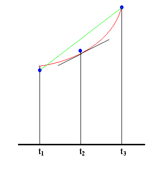
Symmetric Difference Approximation

In the above illustration, the three data points which appproximate the values of the function P at t₁, t₂, and t₃ are shown in blue. The graph of P is drawn in red, and the tangent line to the graph of P at t₂ is drawn in black. We use the slope of the secant line (in green) which connects the data points at t₁ and t₃ to estimate dP/dt at t₂. This is the symmetric difference approximation to the derivative.

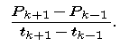
Show that the symmetric difference approximation to dP/dt at t₂ is

where P₁ is the approximate value of P at t₁, and P₃ is the approximate value of P at t₃.

Now we return to testing whether the population of Houston can be modeled by exponential growth.

Use symmetric differences to estimate the rate of growth of Houston in 1900 and in 1950.

Recall from step 1 that one characterization of exponential growth is that the productivity rate is constant. So we want to estimate the values of

and see whether they are approximately constant.

Use symmetric differences to approximate the productivity rates for Houston area population from 1860 to 1970. Why can we not use this method to approximate the productivity rates in 1850 and 1980?
Determine a reasonable constant value k for these approximate productivity rates.
Complete the process of finding an exponential function which models the Houston population data. Compare this function to the one you obtained in step 15.

A final note about symmetric differences

In later parts of this module we will use symmetric differences on data that is not evenly spaced -- in contrast to the Houston population data, which was given every ten years. Nevertheless, we will use the same method of approximating the derivative and continue to call it a "symmetric difference approximation." So, suppose that our data set contains approximations P₁, P₂, ..., P_n to the values of a function P(t) at t₁, t₂, ... ,t_n. We will approximate the value of dP/dt at t_k (for k not equal to 1 or n) by

modules at math.duke.edu