Least Squares
Part 2: Modeling the cancer
death data
In Part 1 of this module,
we saw that we could find the coefficients m and b of the least squares
line y = mx + b by finding the projection p of the data vector y
on the span W of the vectors 1 and x in R9. In
fact, p = b1 + mx -- that is, the coefficients are
also the coordinates of p with respect to the basis {1, x}
of W.

We saw in Part 3 of the
Orthogonality module that the projection p is UUTy,
where U is a matrix whose columns are an orthonormal basis for W. In this
part we find p this way. Of course, our given basis {1, x}
is not orthonormal, so we have to start by constructing U.
- Enter the data vectors
x and y, as well as the vector 1 (called one
in your worksheet). Following the data entry step, you will find code for
constructing U. Explain the steps of this construction carefully.
- Find the projection p.
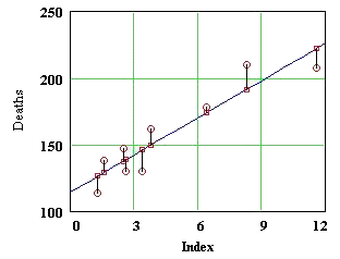
The entries of this vector are related to something in the figure above,
which shows the original data points and the line y = mx + b. Explain carefully
where the entries of p are found in the figure.
modules at math.duke.edu
