The Equiangular Spiral
Part 2: Measuring a Spiral Seashell
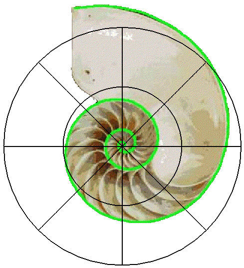
The following figure shows a cross-section of a nautilus shell with a superimposed polar coordinate grid. The outer spiral of the shell has been traced with a green curve. Our objective in this section is to determine a formula for the green curve by measuring the r coordinates of points on the curve and then fitting to the measured points.

You may do your measurements with a ruler marked either with metric units (centimeters and millimeters) or with English units (inches and fractions of inches). These measurements may be done either on your computer screen or on a printed copy of this page, whichever you find more convenient.
No matter how carefully you measure, your results will not be highly precise. First, the placement of the center of the grid is somewhat arbitrary. Second the green curve is a rough approximation of the outer curve of the shell. Third, the curve has been drawn with a rather thick line -- you should try to measure consistently to the center of the line.
If you cannot do measurements on the picture, either on screen or on a printed copy, click here.
- Start with the point of the green curve that is on the theta = 0 line and about one-quarter inch (or 6 mm) from the origin. (The actual distance depends on the resolution of your screen or printer and may differ somewhat.) Measure r for this point as carefully as you can, and record the value where indicated in your worksheet. Then move along the curve to theta = pi/4, and measure the next value of r. Continue around the spiral, recording each r value as you find it. You should be able to make two and a quarter complete turns around the spiral, thereby recording a total of 19 distances.
- Follow the instructions in your worksheet to plot the sequence of radial measurements, rn, as a function of the counter n. What sort of growth does this look like?
- Experiment with logarithmic plotting of the data to determine the type of growth.
- Find a formula for a continuous function r = R(t) such that R(n) reasonably approximates the n-th measured radius, rn. [We are calling this function R to distinguish it from the function r(theta) that we will find in the next part of the module.]
- Test your formula by superimposing the graph of R(t) on the plot of the data {rn}. If the fit is not good enough, adjust your formula until it is. When you are satisfied with the fit, move on to the next part.
